Comparing Lagrange and Bezier interpolation
Let's continue our discoveries in Chapter 7 of the Book by discussing my solution to 7.P1.
We have talked the de-Casteljau algorithm before. It is an expensive but numerically stable way to calculate the points on a Bézier curve given it's control Polgon. Just to remember, this is how it is calculated:
Given the points $$\vec{b}_0 ... \vec{b}_n \in \mathbb{R}^m$$, $$t \in \mathbb{R}$$. Set
Then $$\vec{b}_0^n(t)$$ is the point with the parameter $$t$$ on the corresponding Beziér curve.
Another common approach to interpolation is to use Polynoms of degree $$n$$. We than also need some $$t_i \in \mathbb{R}$$ that corresponds to the given $$\vec{b}_i$$, if they aren't given we can just set them so that they are equally distributed betwenn $$[0,1]$$.
Aitken's Algorithm is than defined by
Given the points $$\vec{b}_0 ... \vec{b}_n \in \mathbb{R}^m$$, with corresponding $$t_i \in \mathbb{R}^n$$ and the position of the interpolation $$t \in \mathbb{R}$$. Set
Then $$\vec{b}_0^n(t)$$ is the point with the parameter $$t$$ on the corresponding interpolating Polynom.
The geometric interpretation is the following: We start out with point 0 and 1 and interpolate linearly between them, than we take 1 and 2 and so on. In the next step, we linearly interpolate between the linear interpolations of the last round by blending the one into the other. The degree of the interpolation polynom increses in each step by one.
The differences between de-Casteljau and Aitken's algorithm in each step are quite simple: The first one is a mapping from $$[0,1] \to \mathbb{R}^m$$ while the second one is mapping from $$[t_i, t_{i+r}] \to \mathbb{R}^m$$.
We can provide a straight forward combination of those two algorithms by mapping from the interval $$[ 0\alpha + (1-\alpha) t_i, 1 \alpha + (1-\alpha) t_{i+r} ]$$ with an $$\alpha \in \mathbb{R}_+$$, that is, we linearly interpolate between the two intervals. Let's define a quick helper function:
Using this, the generalized algorithm looks like this
Given the points $$\vec{b}_0 ... \vec{b}_n \in \mathbb{R}^m$$, with corresponding $$t_i \in \mathbb{R}^n$$, a blending factor $$\alpha \in \mathbb{R}$$ and the position of the interpolation $$t \in \mathbb{R}$$. Set
Then $$\vec{b}_0^n(t)$$ is the point with the parameter $$t$$ on the corresponding blend between Bézier and Polynomial interpolation.
The De-Casteljau algorithm is the special case for $$\alpha = 1$$, Aitken's Algorithm is the special case for $$\alpha = 0$$. Here is a plot of a planar interpolation:
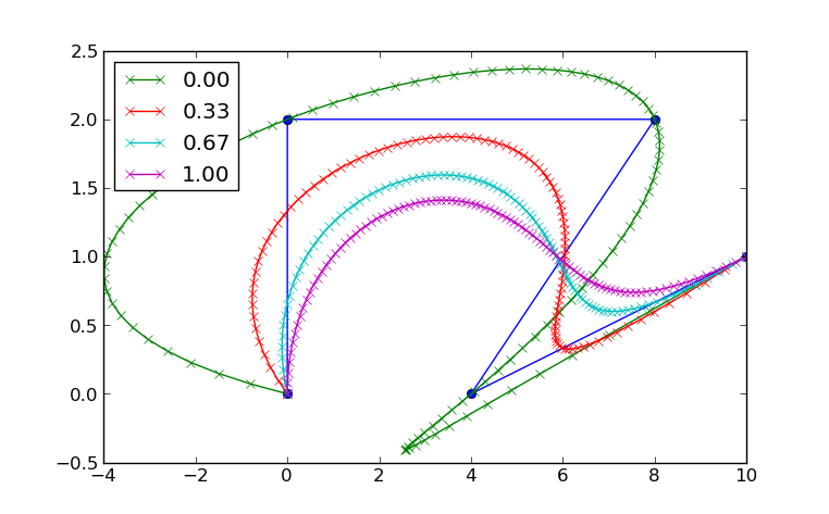
See how the curve for $$\alpha = 0$$ passes through all 4 points. This is a property of Lagrange interpolation (polynomial interpolation). The curve for $$\alpha = 1$$ is the only one that stays in the convex hull of the points; this is a property of Bézier curves.
As always, you can find the complete code for this post in the GitHub repository under chap07. Also, Farin has written a paper on this very topic. You can find it here.