Degree Reduction of Bezier Curves
Continuing with my reading efforts in Curves and Surfaces for GACD by Gerald Farin, I will talk today about a topic that comes up in chapter 6: elevating and reducing the degree of a Bézier curve.
Elevating the dimensionality
First, we start out by proving that the degree of a Bézier curve can always be elevated without the curve being changed.
A curve $$\vec{x}(t)$$ with the control polygon $$B = {\vec{b}_0, \ldots, \vec{b}_n}$$ can be represented as a Bézier curve using the Bernstein Polynomials $$B_i^n$$ as basis:
We will now prove that we can increase the degree from $$n$$ to $$n+1$$ and still keep the same curve, given we choose then new control polygon accordingly.
We start out by rewriting $$\vec{x}(t)$$ as
And now we show that the terms can be rewritten as a sum from 0 to n+1. Let's start with the first term:
Easy. Now the second one
Now, we plug this into the summation formula. We can readjust the summation variables cleverly by noting that we only add 0 terms and we get the formula:
Now all there is to do is to compare the coefficients for old control polygon points and new polygon points and we have our solution: the new points are linear interpolations of the old ones. We can find the new points $$\vec{B}^{(1)}$$ from the old $$\vec{B}$$ by a simple Matrix multiplication:
with the Matrix $$\mat{M}$$ being of shape $$n+1 \times n$$ and looking something like this:
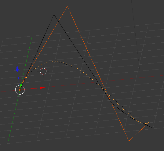
Degree Reduction
The hard work is already done now: It only remains to say that we indeed find the best approximation to our Bézier curve (in the least squares sense) by finding the least-squares solution to the inverse of the system of equations given in the Matrix equation. Therefore, we find the best degree reduced control polygon by
And here is an example from inside Blender. The highlighted objects are the reduced control polygon (n=4) and its Bézier curve. The non highlighted are the originals with one degree higher (5).
As always, you can find the source code for this in the corresponding GitHub project.