Your browser (Internet Explorer 6) is out of date. It has known security flaws and may not display all features of this and other websites. Learn how to update your browser.
X
Red-Black trees

The Red-Black Tree

Another self balancing data structure is the Red-Black tree. What are its properties? First, it is a binary search tree, so the search property is there obviously. And it's other properties? First off, each node has a color associated with it, either red or black, Doh. It then also needs to obey the following rules:

  • The root is black.
  • A red node only has black children.
  • The path from any leaf to the root contains the same number of black nodes than the path from any other leaf to the root.

When we insert a value in the tree, we put it at the right location following the search property and color it red. This might break any of those properties, so we have to make sure they are fulfilled again. I am not gonna lie: Enforcing those rules is complicated, because there are so many combinations of colors the surrounding nodes might have. Checking for them is tedious, but straight forward. In fact Wikipedia lists 5 cases of colors of relative nodes for insertions to be taken into account and 2 simple and 6 non simple cases for deletion. The checks and fixes for the tree are easy and I will not repeat them here. In fact, my own implementation is more or less straight from Wikipedia.

The good thing is that most cases can be handled by only one or two rotations and some local recolorings. There is only one insertion case and one deletion case that needs to traverse the tree upwards again. This makes the Red-Black tree quite a bit cheaper than the AVL tree for those operations. The downside? It is not as strictly balanced.

Number of nodes in the tree

The number of black nodes in any path from leaf to root must be at least $$h/2$$. If we now use the assumption that each subtree of a node $$n$$ must contain at least $$2^{b(x)} -1$$ nodes; $$b(x)$$ is here the number of black nodes from $$n$$ to the root. This is easy to prove by induction.

Together, those two ideas give an estimation:

\begin{eqnarray*}n & \geq & 2^{h/2} - 1 \\ \Rightarrow h & \leq & 2 \log _2(n + 1)\end{eqnarray*}

This is quite a big higher than the AVL tree was, remember? But still logarithmic, which is good.

Let's look at our canonical example as it will look with an Red-Black tree as container:

Our example as red black tree

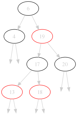
See. In a sense it is prettier than the AVL tree because it has colors! But it is also not so pretty because it is not so well balanced. But you can immediately check that the properties are fulfilled:

  • The root is black.
  • Each red node has only black children (or none).
  • There are always 2 black nodes on each path from leaf to root.

So this is indeed a valid Red Black tree.

We looked at three types of binary search trees by now and we have implementations for all three of them available. What lies closer than benchmarking them?

Benchmarking

For the following tests I used two lists of values:

  • A: the values from 0 to 2999 in random order. No duplicates.
  • B: 1000 random values in the same range including duplicates.

I measured the time to

  • insert all values from A into each container (insert column).
  • delete all values from B from the filled container (delete column).
  • search for all values from B in the filled container (search).
  • construct a sorted list - that is an inorder traversal - from the filled container (iterate).
Tree type insert delete search iterate
BS 36 ms 14.4 ms 8.49 ms 6.49 ms
AVL 117 ms 16.0 ms 6.89 ms 5.39 ms
RedBlack 64 ms 19.8 ms 6.9 ms 5.52 ms

The timings are as expected: insertion and deletions goes fastest in the binary search tree (BS) because it doesn't need to do anything special. The AVL tree is slowest because it is most aggressive with balancing the tree. It gains ground on the red-black tree on deletion though: maybe the extra work on deletion is not so bad for the AVL tree; note it is still slower than the binary search tree.

Funny enough, searching and iterating is not really much faster in the AVL tree compared to the red-black tree. That shows why red-black trees are used so often: they are an excellent trade off in insertion/deletion speed compared to search speed.

Conclusion

Today, I presented you a very, very brief look at Red-Black trees. We only talked through the properties and looked at one example. I also finished the series with a benchmark for all three implementations.

You can find the implementations in the GitHub repository of mine. Take them for a spin yourself! If you are more of the theoretical type, go devour the Wikipedia page on Red-Black trees instead.

This concludes my series on binary search trees. If I feel so inclined, I might make another tree topic about B-Trees which I find particularly interesting.

Spirituality and God

Einstein and Faith

I recently stumbled upon this nice collection of facts about Albert Einstein. The site has plenty of remarkable quotes that show how deeply this man got it and how far he matured in his life. One that resonated especially with me was this remark about the question if God exists:

We are in the position of a little child entering a huge library filled with books in many languages. The child knows someone must have written those books. It does not know how. It does not understand the languages in which they are written. The child dimly suspects a mysterious order in the arrangement of the books but doesn't know what it is. That, it seems to me, is the attitude of even the most intelligent human being toward God. We see the universe marvelously arranged and obeying certain laws but only dimly understand these laws.

I found the quote translated in German here, I am unsure in which language it was delivered first. This one is supposedly quoted from D. Brian: Einstein – a life, Wiley 1996, p. 186.:

Wir befinden uns in der Lage eines kleinen Kindes, das in eine riesige Bibliothek eintritt, die mit vielen Büchern in verschiedenen Sprachen angefüllt ist. Das Kind weiß, dass jemand die Bücher geschrieben hat. Es weiß aber nicht, wie das geschah. Es versteht die Sprachen nicht, in der sie geschrieben wurden. Das Kind erahnt dunkel eine mysteriöse Ordnung in der Zusammenstellung der Bücher, weiß aber nicht, was es ist. Das ist nach meiner Meinung die Einstellung auch des intelligentesten Menschen gegenüber Gott. Wir sehen ein Universum, das wunderbar zusammengesetzt ist und bestimmten Gesetzen gehorcht, aber diese Gesetze verstehen wir nur andeutungsweise. Unser begrenzter Verstand kann die mysteriösen Kräfte, welche die Konstellationen bewegen, nicht fassen.

I sat through scientific talks that ended with the lecturer preaching his own faith and trying to convert the audience and I also talked to remarkable thinkers that were of the opinion that only secular people could be proper and neutral scientists.

I am not religious. I can resonate with the book parable however and I am deeply interested in the ordering of the books, however, I am all Meh about who put them there. But for me this quote of Einstein is the one reason why I would be religious and the one reason why I can understand if people are. It also builds a bridge between science and religion showing that truly the one can nurture the other. Coexistence is not only possible, but natural.

Chaos Communication Camp Day 1

Transparent Proxies and Hackers

This is it! Me and huega have finally arrived in Berlin at 2am this morning at the Camping ground for the Chaos Communication Camp 2011. The wetter was less than awesome, rain since a few days. But luckily, our friends from VO1d got awesome and recycled the pavilions that the wetter broke into a half-dome which is super stable and water proof. It provided shelter for the night.

The dome the vo1d people build

We stayed in bed till the wetter got better. There was hardly any rain today and we had some time to get our own tent going. Not so pimp, but it works.

text

With the basics in place, I could turn to my projects...

Transparent proxy

My goal is to set up a transparent proxy for a single user on my box. That is, whenever a user for example accesses the web, I want his accesses to go through a program on my choosing before going out to the web. This is easy enough to set up in Mac OS X:

sudo sysctl -w net.inet.ip.scopedroute=0
sudo sysctl -w net.inet.ip.forwarding=1

sudo ipfw add 40 fwd 127.0.0.1,1234 tcp from any to any 80 uid paul

This sets up that any traffic by user paul that leaves the computer on port 80 would instead be transferred to localhost, port 1234. Except that it doesn't work. Every time, a packet hits this rule, the computer freezes and no other network traffic is handled. Stripping the last two words from the rule and everything works as expected - but of course for all users and not only for paul. This is not what I want.

I have no explanation for the behaviour. It could be a PEBKAC, but I guess it is a bug in the ipfw tool or the firewall implementation of Snow Leopard. The feature is esoteric enough to pass unnoticed. That doesn't help me though, so I continue setting up a virtual box with Linux to try the very same thing there.

Some fancy new features of C++11

C++ 2011 bag of features

The now finalized new standard for the C++ language brings a bag of new and exciting features to C++. It will reduce verboseness and increase performance in a lot of areas. Of course, it has to stay backwards compatible; that is why some of the bigger and uglier flaws of C++ can't be changed. Still, it improves the language dramatically. Here is what I will enjoy the most.

Auto and container iterate

Following code annoys me:

std::vector<int> a;
for (std::vector<int>::iterator i = a.begin(); i != a.end(); ++i)
   cout << (*i) << endl;

It raises the following question: if I know that a is a vector and I know that a.begin() returns an iterator, why do I have to retell this to the compiler? It knows this as well. Luckily, it is no longer needed:

for (auto i = a.begin(); i != a.end(); ++i)
   cout << (*i) << endl;

Nearly a pleasure to read. For even shorter code, I would have used boost::foreach in the past, but this is now also included into the language. And it's syntax is pretty:

for (auto v : a)
   cout << v << endl;

This will print all values inside the container a. Since a is a vector of int s, v will be an int as well.

Initializer lists

C++ allows now to initialize even complex types with initializer lists similar to how C did things. This will also replace constructor syntax with brackets for the most parts and it is a good thing, because initializations look more like initializations and not like function calls. The following is valid in C++0x:

std::vector<int> a = { 1, 2, 3, 4, 5 };

You no longer have to mess around with push_back all over the place.

Putting the features together, we can write nice non-verbose code. The following complete C++ program prints the contents of a std::map.

#include <iostream>
#include <map>

using namespace std;

int main(int argc, char const *argv[]) {
   map<string,int> cmap {
      {"Hello", 5},
      {"World", 10}
   };

   for (auto k : cmap)
      cout << k.first << ":" << k.second << endl;

   return 0;
}

static_assert and variadic templates

static_assert can be used to write asserts on compile time. Widelands uses this in some places to make sure that space optimization that assume some sizes of datatypes do not break down. In the past, you had to jump through some loops to get this working. Now it is as easy as

static_assert(sizeof(long) == 8, "Your long, it is too small!");

Variadic templates are templates that can take a variable number of arguments. They are used to implement std::tuple for example.

But they can also be used to implement self recursive templates that can consume input one element at a time at compile time. For example the following program does precisely nothing at run-time but converts a binary string to an int at compile time:

template <char... digits> struct _2bin;

template <char high, char... digits> struct _2bin<high, digits...> {
   static_assert(high == '0' or high == '1', "no binary number!");
   static int const value = (high - '0') * (1 << sizeof...(digits)) +
         _2bin<digits...>::value;
};

template <char high> struct _2bin<high> {
   static_assert(high == '0' or high == '1', "no binary number!");
   static int const value = high - '0';
};

int main(int argc, char const *argv[])
{
   const int a = _2bin<'1', '1', '1', '1', '1', '0'>::value;
   static_assert(a == 62, "Didn't work out :(");

   return 0;
}

Extendable literals

This is still not supported in gcc 4.6, but the standard allows to create an operator for literal suffixes. The following is allowed by the standard but does not compile currently:

template<char... digits> constexpr int operator "" _b() {
    return _2bin<digits...>::value;
}

int main(int argc, char const *argv[])
{
   const int a = 111110_b;
   static_assert(a == 62, "Didn't work out :(");

   return 0;
}

Note the constexpr. It tells the compiler that it can evaluate this function on compile time and so it will. The operator "" syntax defines a new literal suffix, _b in this case. It allows to write a literal as seen in the definition of a. Like all operators in C++, this also basically adds syntactic sugar which makes code easier to read.

Extendable literals are a fun to play around with and allow for a lot of domain-specific gravy in C++ code without run-time overhead. Still, it is more of an esoteric new feature of the language. For the specific problem discussed here - binary literals - you are better off using a compiler extension. Most compilers support binary literals in the form of 0b111110 these days.

Conclusion

C++0x brings a bag of nice features. All of the above except for extendable literals are already supported in GCC 4.6, but you need to pass -std=c++0x as argument on the command line while compiling.

If you want to know more, Wikipedia has a detailed rundown of the new features in C++0x. There are some that I did not discuss here and that I am not so exited about as the ones mentioned.

I am looking forward to seeing all those features become more widespread. As far as I am concerned, I will only program C++0x in the future if I have the choice and I will not weep for superseded features that will slowly vanish into oblivion. Altogether, I feel like the standardization committee did a great job with the new standard, it breathes new live into a language that we are stuck with for years or maybe decades to come.

Generators in C++

Generators in C++

Generators are iterators over things made up on runtime. For example if you ask me about the Fibonacci sequence, I can generate an infinite amount of them by only remembering the two numbers before:

\begin{eqnarray*}F(0) &=& 1 \\ F(1) &=& 1\\ F(n) &=& F(n-1) + F(n-2)\\\end{eqnarray*}

Generators are quite useful for programming. Python has them, Haskell is basically build around them (I think they call them infinite lists). Generating the Fibonacci sequence up to a maximum number maxn looks like this in Python:

def fib(maxn):
    n, ln = 1, 1
    while n < maxn:
        yield n
        n, ln = ln, n + ln

for i in fib(1000):
    print i,

After my last blog post about C++0x features, I was intrigued to write something similar in C++. The corresponding main function also looks very nice with the new container iterate feature:

#include <iostream>

int main(int, char argv**)
{
   FibonacciGenerator k(1000);

   for(auto i : k)
      std::cout << i << " ";
   std::cout << std::endl;

   return 0;
}

So basically, we have a container here called FibonacciGenerator and we iterate over it with the new container iterate feature. For this to work, we have to implement the begin() and end() functions in the container and the values those functions return must implement operator++, operator* and operator!=. This goes something like this:

class FibonacciGenerator {
private:
   struct generator {
      generator(int n) : _n {n}, _ln{0} {}

      int & operator*() {
         return _n;
      }

      bool operator!=(const generator & other) const {
         return _n <= other._n;
      }

      generator& operator++() {
         int temp = _ln + _n;
         _ln = _n;
         _n = temp;
         return *this;
      }

      private:
         int _n, _ln;
   };

public:
   FibonacciGenerator(int maxn) : _maxn{maxn} {}
   generator begin() const {
      return generator(1);
   }
   generator end() const {
      return generator(_maxn);
   }

private:
   int _maxn;
};

The implementation is quite straightforward: All the (not very heavy) lifting is done in the generator. The inequality compare checks if the current number is bigger than the one of the other iterator. If this becomes true, the loop in main will terminate. The dereference operator returns the current number and the increment operator calculates the next. The container itself only contains the begin and end function which are called by the container iterate syntactic sugar.

Note that generators are nothing new. You can write them in exactly the same way in C++03. But somehow, the new Pythonic container iterate feature triggered me for the first time to think about them in C++.

Degree Reduction of Bezier Curves

Degree Reduction of Bezier Curves

Continuing with my reading efforts in Curves and Surfaces for GACD by Gerald Farin, I will talk today about a topic that comes up in chapter 6: elevating and reducing the degree of a Bézier curve.

Elevating the dimensionality

First, we start out by proving that the degree of a Bézier curve can always be elevated without the curve being changed.

A curve $$\vec{x}(t)$$ with the control polygon $$B = {\vec{b}_0, \ldots, \vec{b}_n}$$ can be represented as a Bézier curve using the Bernstein Polynomials $$B_i^n$$ as basis:

\begin{equation*}\vec{x}(t) = \sum_{i=0}^{n} \vec{b}_i B_i^n(t)\end{equation*}

We will now prove that we can increase the degree from $$n$$ to $$n+1$$ and still keep the same curve, given we choose then new control polygon accordingly.

We start out by rewriting $$\vec{x}(t)$$ as

\begin{eqnarray*}\vec{x}(t) &=& (1-t) \vec{x}(t) + t \vec{x}(t) \\ &=& \sum_{i=0}^n (1-t) \vec{b}_i B_i^n (t) + \sum_{i=0}^n t \vec{b}_i B_i^n (t)\end{eqnarray*}

And now we show that the terms can be rewritten as a sum from 0 to n+1. Let's start with the first term:

\begin{eqnarray*}(1-t) B_i^n (t) &=& (1-t) \frac{n!}{(n-i)! i!} t^i (1-t)^{n-i} \\ &=& \frac{n + 1 - i}{n + 1} \frac{(n+1)!}{(n+1 -i)! i!} t^i (1-t)^{(n+1)-i} \\ &=& \frac{n+1 - i}{n+1} B_i^{n+1}(t)\end{eqnarray*}

Easy. Now the second one

\begin{eqnarray*}t B_i^n(t) &=& t \frac{n!}{(n-i)! i!} t^i (1-t)^{n-i} \\ &=& \frac{i+1}{n+1} \frac{(n+1)!}{(n+1)!(i+1)!} t^{i+1} (1-t)^{n-i} \\ &=& \frac{i+1}{n+1} B_{i+1}^{n+1} (t)\end{eqnarray*}

Now, we plug this into the summation formula. We can readjust the summation variables cleverly by noting that we only add 0 terms and we get the formula:

\begin{eqnarray*}\vec{x}(t) &=& \sum_{i=0}^{n+1} \frac{n+1-i}{n+1} \vec{b}_i B_i^{n+1} (t) + \sum_{i=0}^{n+1} \frac{i}{n+1} \vec{b}_{i-1} B_i^{n+1} (t) \\ &=& \sum_{i=0}^{n+1} \Big( \big(1 - \frac{i}{n+1}\big) b_i + \frac{i}{n+1} b_{i-1}) \Big) B_i^{n+1} (t)\end{eqnarray*}

Now all there is to do is to compare the coefficients for old control polygon points and new polygon points and we have our solution: the new points are linear interpolations of the old ones. We can find the new points $$\vec{B}^{(1)}$$ from the old $$\vec{B}$$ by a simple Matrix multiplication:

\begin{equation*}\mat{M} \vec{B} = \vec{B^{(1)}}\end{equation*}

with the Matrix $$\mat{M}$$ being of shape $$n+1 \times n$$ and looking something like this:

\begin{equation*}\mat{M} = \begin{pmatrix} 1 & & & \\ \frac{1}{n+1} & 1- \frac{1}{n+1} & & \\ & \frac{2}{n+1} & 1- \frac{2}{n+1} & \\ \vdots \\ & & \frac{n}{n+1} & 1- \frac{n}{n+1} & \\ & & & 1 \end{pmatrix}\end{equation*}

Degree Reduction

The hard work is already done now: It only remains to say that we indeed find the best approximation to our Bézier curve (in the least squares sense) by finding the least-squares solution to the inverse of the system of equations given in the Matrix equation. Therefore, we find the best degree reduced control polygon by

\begin{equation*}\vec{B} = (\mat{M}^T \mat{M})^{-1} \mat{M}^T \vec{B}^{(1)}\end{equation*}

And here is an example from inside Blender. The highlighted objects are the reduced control polygon (n=4) and its Bézier curve. The non highlighted are the originals with one degree higher (5).

Reduced control Polygon and original + splines

As always, you can find the source code for this in the corresponding GitHub project.

Better Navigation

Better Navigation on this Blog

I just added a calendar widget on each page where it makes sense here. I am not sure how useful it is, so I will try it out for a while and remove it again if it makes no sense.

I also improved the blog archive list in the right navigation bar. I was inspired by something I saw on Guido's blog, namely a folding tree view. I am aware that most blogging tools like Wordpress have this feature build in, but I realized the first time how useful it is on Guido's page. So I copied it. Turned out that you only need a little bit of Javascript and CSS. I basically followed the short but concise tutorial by David Herron. I only needed very few adjustments, but they were trivial thanks to the beauty that is jQuery.