A Linear Algebra View on Least Squares
Last time, we introduce the least squares problem and took a direct approach to solving it. Basically we just minimized the $$y$$-distance of a model to the data by varying the parameters of the model. Today, we find a completely different, but very neat interpretation.
Suppose we have the following problem: There is a set of linear equations without a solution, e.q. a matrix $$\mat{A}$$ and a vector $$\vec{b}$$ so that no vector $$\vec{x}$$ exists that would solve the equation.
Bummer. What does that actually mean though? If we use every possible value of $$\vec{x}$$ in this equation, we get essentially all linear combinations of the column vectors of $$A$$. That is a span of vectors. That is a subspace. So, $$\vec{b}$$ is not in our subspace, otherwise we would find an $$\vec{x}$$ that would solve our linear equation.
Here is a visualization in 3D when A is a two dimensional matrix:
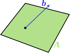
The column space of the matrix is a plane and $$b$$ is not in the plane. A natural question now is: what is the vector in the column space of $$\mat{A}$$ that is the best approximation to $$b$$. But what is a good approximation? Well, how about the Euclidian distance between the endpoints of the vectors. If we choose this criteria, there is a simple solution: the projection of $$\vec{b}$$ to $$\mat{A}$$ will give the best approximation. Here is another image:
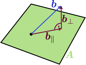
We have decomposed $$\vec{b}$$ into its best approximation in $$\mat{A}$$ which we call $$\vec{b_\parallel}$$ and a component that is orthogonal to it called $$\vec{b_}\perp$$. At the end of the day, we are interested in a best approximated solution to our original equation, so we are not really interested in finding $$\vec{b}_\parallel$$, but rather an $$\vec{x^*}$$ so that
Lets look for an equation for this $$\vec{x}^*$$. We will start out by using that the two components of $$\vec{b}$$ are perpendicular to each other. And we will also express $$\vec{b}_\perp$$ through vector addition.
Since $$\vec{x}^*$$ can't be zero, the term in parenthesis must be. This directly yields the least squares formula again:
Conclusion
We did the exact same thing as in the last post, but this time we took another approach and quite a different world view on the problem. The least squares solution came up very naturally here and with a very simple geometric interpretation (at least in the 3d case, the approach is also valid for other dimensions though).
The last iteration of this series will take a look at least squares in statistical models.