Your browser (Internet Explorer 6) is out of date. It has known security flaws and may not display all features of this and other websites. Learn how to update your browser.
X
Revamping the site

Revamping the site

Welcome back to my new and drastically improved website! In the last few weeks I worked to improve all aspects of the site for my own benefit mostly, but also for yours! So what you see here is all new: new design and new deployment technology. Only the content hasn't changed.

New Technology

Okay, I didn't blog as much as I wanted to in the past. There were numerous reasons, but lack of content wasn't the dominating one. The biggest problem was that the old django site didn't allow to quickly write down and preview a blog post in Vim. There was always a mental barrier to get started writing my thoughts down.

So I switched from Django to Blogofile which is basically a fancy static web site generator written in Python. So instead of generating the HTML on the fly on the server it is generated offline and then uploaded to the server. This has a number of advantages like enhanced security, quicker deployment and serving of the site. It also means I have the whole site under version control at all time and can carry it around with me wherever I go.

The disadvantages is that there is no longer any dynamic behaviour on the server site possible, so no fancy session support or contact forms. I have some ideas how this could be monkey patched into this, but for the moment I can live without that. I also believe that there is quite a lot possible with using javascript, so I might not need server site scripts at all.

The site is basically at the same functionality level than the Django site I used before. Especially code and LaTeX integration are top notch (for me). We still have no comments, but I hope to get Disqus Integration rolling sometime soonish.

New Layout

I was a bit sick of my old layout. It was ugly. The reason it was ugly is that I have no skill with CSS and HTML. Yep, I know the technical parts of it, but I am not a good designer, have no eyes for fonts, colors and so on. So I decided to spend some bucks and support a freelancing designer named kubasto on themeforest.

I personally find the dark black-yellow design gorgeous. And kubasto knows his trade: He included some javascript snippets to integrate with twitter, facebook and what not. I had some work to do to convert his code from PHP back to Mako Templates, but I think I have ironed out the most awful bugs by now.

What's next?

I revamped the blog for a reason: I finally want to do what I promised to do when I started this thing. I also need a page for some of my personal projects (e.g. UltiSnips) and as I am currently revamping a lot of topics from statistics, machine learning and computer science I want to provide short blog posts with explanations and code for others (and myself in a few years) to follow and learn from. Let's hope I deliver this time!

Blender 2.5 and Blossoms

Using Blender 2.5 as Visualization Tool

For my PhD work I use Blender as visualization tool. It suits me because it uses python for scripting and is very flexible. I can also use it directly to navigate my results and render them for publication.

Blender has seen a major overhaul with version 2.5, nearly everything works differently: the GUI has changed, the internal python API has changed, the feature set has changed (grown mostly). Getting my stuff from Blender 2.4 to Blender 2.5 will be a major undertaking which I do not want to tackle now. However, I feel that it is about time to start learning it, because before I give my work to my successor, I should really port it to the current blender version.

Reviewing Interpolation

Also for my work, I am currently skimming through the book Curves and Surfaces for GACD by Gerald Farin. I need some inspiration for a better representation of my surfaces. It is a great book. If you are interested in programming 3D graphics or interpolation you should really get it.

The programming problem P1 in chapter 3 is the following:

Let three points be given by

$$$\vec{b}_0, \vec{b}_1, \vec{b}_2 = \begin{bmatrix}0 \\ 0\end{bmatrix}, \begin{bmatrix}40 \\ 20\end{bmatrix}, \begin{bmatrix}50 \\ 10\end{bmatrix}.$$$

For s = 0, 0.05, 0.1, ...1 and t = 0., 0.05, 0.1, ..., 1 plot the points b [s,t].

The function b is defined earlier in the book and is called a bivariate Blossom. It is defined by the following equation:

$$$\vec{b}[s,t] = (1-t)(1-s) \vec{b}_0 + [(1-t)s + t(1-s)]\vec{b}_1 + s t \vec{b}_2$$$

Using the brevity of Python, this results in this wonderful class definition:

 1
 2
 3
 4
 5
 6
 7
 8
 9
10
11
12
import numpy as np

class Blossom(object):
    def __init__(self, p1, p2, p3):
        self._pts = np.asarray([p1, p2, p3])

    def __call__(self, t, s):
        return np.dot((
            (1-t)*(1-s),
            (1-t)*s+t*(1-s),
            s*t),
            self._pts)

Putting it together

So I put together a python script that can be loaded and executed in Blender 2.5. It sets up a menu that is shown in the 3D View whenever a mesh with exactly 3 vertices is selected. It allows you to set the range for s and t and updates the Blossom mesh with the calculated points.

The final result looks something like this:

the menu is on the left, the Polygon and the Blossom is on the right

It took a while to put the script together: The documentation of the new python API is not very complete at the moment and googling for Blender 2.5 specific help is not trivial. I hope this script gets someone else jump started. You can find the python script here and the blender scene which also includes the python script here.

Update: The code is now also available on GitHub.

Adding discussions to the blog

Discussions using Disqus

I just introduced a new feature to this blog which is something I wanted to have for a very long time: Discussion threads. I already talked about this in my original revamping the site article and I basically went with what I have had planed.

So this site is now using the Disqus service for handling comments. This means you can use basically any account you already have to comment on my work here on the blog or just comment anonymously. I wonder how good the spam handling of Disqus is.

Implementation

From an implementers standpoint, the Disqus API is very straightforward and well documented. Essentially you just define some javascript variables, then include some scripts from disqus.com in your site and you're done.

The control is not as fine tuned as I would have liked though. For example you do not get the chance to iterate over every comment and output your own HTML code. I do not doubt that it is possible by looking at the javascript from Disqus, but it is not officially supported.

Style

However, the wonders of CSS gave me the power to reformat their HTML output to match the prettiness of black and yellow. I had to redefine some formatting that where already set by my styles - then overwritten by the Disqus style sheet for their elements - to match my style again. A little cumbersome, but easy.

I mostly looked at the rendered page source to figure out which classes I needed to format in the CSS, but there is also a nice blog post on onbloggingwell.com on this very topic which was useful.

So, I hope to read some comments in the future! I will go ahead and make the first test post as anonymous myself right away, you can bet on this :).

New parser for UltiSnips

UltiSnips got a new parser

UltiSnips is the Vim plugin for Snippets I have started. It has become fairly successful with quite some people contributing snippets and code to it. I use it myself on a daily basis and can't remember how I did things before it was around. For example, I have the following snippet defined to start blog posts:

snippet blog "Blog Post Header" b
---
uuid: `!p if not snip.c: snip.rv = uuid.uuid4().hex`
date: `!p snip.rv = dt.datetime.now().strftime("%Y/%m/%d")`
type: ${1:article|quote|link|image|video|audio|custom}
title: ${2:Awesome, but short title}
tags: ${3:tag1,tag2}
---

${0}
endsnippet

The first line introduces this as a snippet definition, while the last line ends it. All between is pasted into my text when I type blog followed by a <Tab>. There is some special syntax:

  • The parts starting with backticks are python interpolated code; that is the first line will become a UUID, the second the current date.
  • The parts starting with ${<number> are tabs. They get selected and when I expand the snippet. I overwrite them my own text, then, by pressing <C-j> I quickly jump to the next tab which is then selected so I can overwrite it.

In toto, UltiSnips spares me to remember a lot of Syntax (like the various article types my blog supports) and a lot of manual work (like putting in the date or creating a UUID). I love it.

The purpose of parsing

When <Tab> is pressed, UltiSnips must learn where the snippet needs to be inserted and where the individual Text Objects (tabs, python code, shell code, vimL code, mirrors, transformation or escaped chars) end up in the text file the user is writing. This needs to be done by learning first where the text objects are inside the snippet and how they relate to each other (e.g., tabs can also be inside default text of other tabs). For this, parsing of the snippet is needed.

The original approach was to use a bunch of regular expressions to find individual Text Objects inside a snippet. This has a number of downsides, the two biggest are that

  • the snippet syntax is not regular.
  • the snippet syntax may contain ambiguity

See this example:

$1 ${1:This is ${2:a default} text} $3 ${4:another tabstop}

The first point is exampled by the 1 tabstop: regular parsing is out of the picture here, because you need to count the { and } to make sure you do not take too little or too much text into your tabstop.

The ambiguity is with the $<number> syntax: The first $1 is a Mirror (a text object that simply repeats the contents of a tabstop), because a tabstop definition appears later in the snippet. The $3 however is a tabstop without default text as there is no proper tabstop definition for 3, so the $3 could be replaced via ${3:} or ${3} and the snippet would behave exactly the same.

Never the less, we had a regular parser for a while now and jumped through many rings to support the cases I just mentioned. Not any more.

The new approach

This the what the new algorithm does:

  1. Tokenize the input text with a context sensitive lexer. The lexer checks for each position in the string which token happens to start here. If one potential token is found, it is parsed according to its own rules.
  2. Iterate through all tokens found in the text.
    1. Append the token and its parent to a list of all tokens in the snippet. As we recurse for tabstops (see next point) this builds a list of tokens in the order they appear in the text.
    2. If the token is a tabstop, recurse the algorithm with text being the default text of the tabstop and parent being the tabstop itself.
    3. If the token describes a text object that has no immediate reference to other tabstops (e.g. Python code interpolation, shell code interpolation or escaped special characters) create the text object and link it to its parent.
  3. When the whole snippet is traversed, do the finalizing touches for the list of all tokens and their parents:
    1. Resolve the ambiguity. As we have seen all tokens by now and already instantiated all easily identifiable tabstops we can go through all the $<number> tokens in order and decide if they are a tabstop (first appearance) or a number (a tabstop is already know for this number) and create them accordingly.
    2. Create objects with links to tabs. Transformations take their content from a tabstop. Now, since all tabs are created, we can traverse the list of tokens again and create all the transformations and pass them their proper tabstop. Also, only now can we detect if a transformation references a non existing tabstop.

You can find the implementation of the new parser in the _TOParser class and the implementation of the lexer in the new Lexer.py file.

The de Casteljau Algorithm

The de Casteljau Algorithm

This is a follow up to Blender and Blossoms.

The de Casteljau Algorithm is a recursive way to calculate the Point on a Bézier curve given its control polygon $$P = \{ \vec{b_i} \}$$ consisting of the Points $$b_i$$. It is defined as follows in the Book:

Given the points $$\vec{b}_0 ... \vec{b}_n$$, $$t \in \mathbb{R}$$ and a function $$f(t): \mathbb{R} \to \mathbb{R}$$. Set

\begin{eqnarray*}\vec{b}_i^0 & := & \vec{b_i} \\ \vec{b}_i^r & := & (1-f(t)) \vec{b}_i^{r-1} + f(t)\,\vec{b}_{i+1}^{r-1}(t)\end{eqnarray*}

Then $$\vec{b}_0^n$$ is the point with the parameter $$t$$ on the corresponding Beziér curve.

So this is essentially a recursive definition: Starting from $$n$$ points, we always combine two of them and remain with $$n-1$$ points. We continue this scheme until only one point is left. This is the point on the curve for the value $$t$$.

Implementation

The de Casteljau Algorithm is short and beautifully implemented:

import numpy as np

class DeCasteljau:
    def __init__(self, *pts, func = lambda t: t):
        self._b = np.asarray(pts, dtype=np.float64)
        self._func = func

    def __call__(self, t):
        b, n = self._b, len(self._b)
        for r in range(1,n):
            for i in range(n-r):
                b[i] = (1-self._func(t))*b[i] + self._func(t)*b[i+1]

        return b[0]

And this is how it looks.

Blender screenshot of polygon with bezier curve

The orange curve is the defining polygon and the dots are the corresponding beziér curve evaluated for 100 values of $$t \in [0,1]$$ and $$f$$ being the identity.

You can find the complete code in the GitHub repository under chap04.

Anonymous snippets in UltiSnips

Anonymous Snippets in UltiSnips

UltiSnips supports anonymous snippets: they are defined on the spot, expanded and immediately discarded again. They were requested by someone and Ryan implemented them, but I was all Meeeh because I didn't understand for what they could be used.

But I just realized they are in fact awesome: I have a new line in my RestructuredText Vim plugin file:

inoremap <silent> $$ $$<C-R>=UltiSnips_Anon(':latex:\`$1\`', '$$')<cr>

Hitting $ now directly translates into being in inline math mode. How cool is that?

Binary search trees

The binary search tree

Let's suppose you want to keep some data in memory. Occasionally, new items arrive, old items get unimportant and you want to delete them. Adding new items and deleting old should not take long. And you want to be able to traverse the data quickly and in sorted order at all points in time.

Arrays are out, because they would shuffle all the elements around on deletion and insertion. What data structures would you use?

Why not use a binary search tree? It only needs $$\mathrm{O}(n)$$ space and insertion and deletion take on average only $$\mathrm{O}(\log n)$$ time. A pretty good deal?

What is it?

A sample binary search tree

This is one for integers. You can put everything that can be ordered inside a binary search tree, but for simplicity, we will stick with integers.

Our tree has 7 nodes in it, so $$n = 7$$. The root node is 6. See the nodes 19 and 6? They have 2 children: left and right. All nodes also have a parent. There are other nodes with either a left or a right child. There are also some nodes without any children, they are called leafs of the tree.

This is called a binary tree because every node can only have a maximum of two children. But what makes it a binary search tree? If you look closely, you will realize that all children that are to the left of a node are strictly smaller and the reverse for the right site. Look at the 19: 20 is to its right and bigger, 6, 4, 13, 18, 17 are to its left and strictly smaller. And that's all there is to it.

Searching & Insertion

This property makes it easy to check if a value is inside our tree. For example, if you want to know if 12 is in the tree you do the following:

  • Start at the root: 12 > 6 so go right,
  • 12 < 19 so go left
  • 12 < 13 so go left again... Ups.

There is no node here. Well, 12 is not in our tree, is it? But if you would want to insert it, you would do it right here, as left child of 13.

Let's look at the python code for those two operations:

def search(node, key):
    if node is None: return None
    if node.key == key: return node
    return search(node.l, key) if key < node.key else \
           search(node.r, key)

search(root_node, 12)  # None, for our case

def insert(node, key):
    if node is None: return Node(key)

    if key <= node.key:
        node.l = insert(node.l, key)
        node.l.parent = node
    else:
        node.r = insert(node.r, key)
        node.r.parent = node
    return node

insert(root_node, 12)

Note that we also do some house holding that the links between children and parents are valid after insertion.

Deleting

Deleting an item is a bit hairy, but there are only three cases:

  • Delete a leaf: Just remove it and you're done. Remember to break the links to its parent though!
def delete_leaf(n):
    if n.parent.l == n:
        n.parent.l = None
    else:
        n.parent.r = None
  • Delete a node with one child: we essentially remove this node from the chain by linking its parent to its child.
def delete_node_with_one_child(n):
    child = n.l or n.r

    if n.parent.l == n:
        n.parent.l = child
    if n.parent.r == n:
        n.parent.r = child
    child.parent = n.parent
  • Delete a node with two children. This is the most difficult one. Look at 19, how could you remove this from the tree? Well, we have to keep the ordering property. So the only two values that we could use in this position that would keep the property are 18 and 20. Those are the biggest item in its left subtree (18) and the smallest item in its right subtree (20). And this is always the case! Which one should we pick? It doesn't matter, but picking one at random will help distribute the items in our tree evenly.

    Now all that is left to do is to delete the node we took the value from.

import random

def biggest_successor(node):
    if node.r:
        return biggest_successor(node.r)
    return node

def smallest_successor(node):
    if node.l:
        return smallest_successor(node.l)
    return node

def delete_node_with_two_childs(n):
    child = smallest_successor(n.r) if random.choice((0,1)) == 0 \
            else biggest_successor(n.l)

    n.key = child.key
    delete_node(child) # could have one or zero children

Traversing the Tree

Now how about getting at the elements in sorted order? We would need to start at the leftmost element in the tree because it is the smallest. The next bigger one is the smallest element in its right subtree. We can express this in a recursion quite nicely:

def iter_tree(node):
    if node.l:
        for k in iter_tree(node.l):
            yield k

    yield node

    if node.r:
        for k in iter_tree(node.r):
            yield k

list(root_node) # -> [4, 6, 13, 17, 18, 19, 20]

Is it a deal?

So we have a nice data structure now, should we use it? Yep. Can we achieve better? Not in the average case. Is is good for all cases? Well, just imagine your data arrives already in sorted order:

Tree becomes a link list on sorted insertion
Rotated to save some space. And it sorta looks like a linked list.

Terrible! Gone is our $$\mathrm{O}(\log n)$$ search time (it is $$\mathrm{O}(n)$$ now). And with it the nice performance of inserts and deletions. What can we do about it? There are some more advanced trees that are able to keep themselves balanced, that means that there are around the same number of nodes in each subtree of each node. We will look at AVL Trees and Red-Black Trees in future installments of this series.

Conclusion

We took a quick glance at binary search trees, how they work and why they are useful. We discussed how easy insert is and that deletion is quite straightforward, but there are many different cases. We also looked at python snippets that implemented the functionality we talked about.

If you want to know more you can either hop over to Wikipedia and read it up for yourself. Or, you can watch the excellent computer science lectures by Dr. Naveen Garg about data structures - especially trees.

Or you could check out the source code for this post on github. There you will find my implementation of a binary search tree and also the visualization routine I used to make the images of our tree here.

AVL Trees

The AVL Tree

Last post we looked at the Binary Search Tree in some detail and we found that it is a pretty good data structure. We also found that it behaves like a linked list and looses its good properties when we insert items in sorted order. Let's work on this and check out a tree that is auto balancing: the AVL tree.

The AVL tree is a binary search tree with one new property: in each node, the height of the left subtree and the height of the right subtree must only 
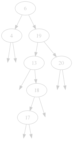
differ by 1 (or zero). That's all there is to it. Let's look at the binary search tree example we saw the last time and check out what needs to be done to make it a AVL tree.

A bst with heights and height balances

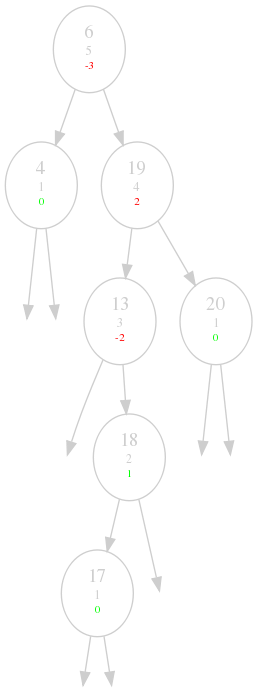
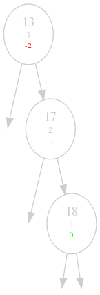
The keys are still written in bigger font size, but I now added two more properties: the smaller numbers in grey is the height of the node. For a node $$n$$, with children $$l$$ and $$r$$ the height $$h(n)$$ is simply defined by

\begin{equation*}h(n) = 1 + \mathrm{max}\Big( h(l), h(r) \Big)\end{equation*}

The colored number is the height balance of a node, which is just the height of its left subtree minus the height of its right subtree. So for example the node 13 has no left subtree, so $$h(l)$$ = 0, the node 18 has height 2, so $$h(r)$$ = 2, this results in a height balance of -2. The numbers are green when they do not violate the AVL property, otherwise they are red.

So what do we need to do to fix the 13 for example? Intuitively, we would like the 13 to go down and the 18 and 17 to come up in some kind of way. But obviously, we need to keep the ordering of the binary tree. The solution is quite simple, first, we do a right rotation with the 18 as root, then we do a left rotate with 13 as the root:

Step 1: right rotate with 18 as root
Step 1: 17 moved up and 18 moved down.
Step 2: left rotate with 13 as root
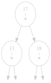
Step 2: 17 moved up and 13 moved down and everything is balanced.

So what is a rotation? For example the left rotation with $$P$$ as root looks like the following. $$R$$ is the right child of $$P$$.

  • $$P$$ becomes the left child of $$R$$
  • $$R$$'s left child becomes $$P$$'s right child

That basically means that $$P$$ comes down while $$R$$ goes up. The right rotation looks the same, but right and left swapped.

What changes for the handling of the tree? Searching and traversing stays the same, it is a binary search tree after all. What about insertion and deletion?

Insertion

Insertion is simple: we just insert the node where it belongs, but than we have to make sure that the AVL property is not violated anywhere. It isn't automatically violated after insertion, but if it is, it can only be violated in one node which is on the path we took while going down the tree. We rebalance this node and are done.

def _just_inserted(self, node):
    "Node was just inserted into the tree"
    par = node.parent
    while par:
        self._update_height(par) # Recalculate the height of the parent
        if abs(par.height_balance) > 1:
            self._rebalance(par) # Rebalance the one node and stop
            break
        par = par.parent # Otherwise continue with parent

    return node

Deletion

Deletion is also easy: The case of a node with two children doesn't change and the deletion in the other cases are just the same. But the height of all the nodes on the path we took down to the nodes might have changed, so we have to check for this and rebalance accordingly. If we encounter a node on our way up that has not changed height, we can stop checking because the nodes above it will not feel any difference.

def _delete_leaf(self, n):
    par = n.parent
    BinarySearchTree._delete_leaf(self, n)
    self._rebalance_till_root(par)

def _delete_node_with_one_child(self, n):
    par = n.parent
    BinarySearchTree._delete_node_with_one_child(self, n)
    self._rebalance_till_root(par)

def _rebalance_till_root(self, node):
    while node and self._update_height(node):
        node = node.parent if \
           abs(node.height_balance) <= 1 else self._rebalance(node)

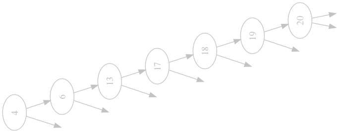
That's all there is to it. Let's repeat our ending experiment from the last time and insert our values in sorted order in our shiny new data structure:

The final AVL-Tree of our example

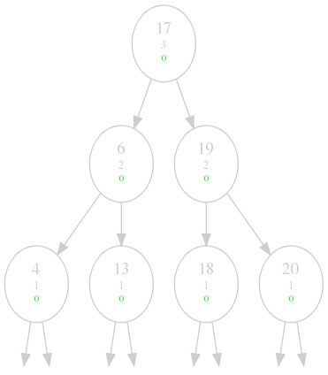
Perfect. But how good is it in the general case?

Number of nodes in the tree

Given $$m$$ nodes, what will be the height of the tree be like? Well, it will likely be some kind of logarithm $$m$$. Let's check this more closely.

Let's define $$n(h)$$ to be minimal number of nodes in a tree of height $$h$$. There is an easy formula for that: the smallest number of nodes is when the left subtree has an height of h-1 and the right h-2, so

\begin{equation*}n(h) = n(h-2) + n(h-1) + 1\end{equation*}

I will state that the following is true and proof it by induction later on.

\begin{equation*}n(h) \geq c^{h-1}\end{equation*}

The question is, what will the biggest $$c$$ be that still solves this inequality? Let's solve for c:

\begin{eqnarray*}(h-1) \log c & \leq & \log n(h) \\ c & \leq & \exp \Big\{ \frac{\log n(h)}{h-1} \Big\}\end{eqnarray*}

Here are some numbers:

h $$n(h)$$ max $$c$$
3 4 2
4 7 1.9129
7 33 1.7910
20 17710 1.6734
50 32951280098 1.6392698637801975

Let's do the induction finally. We assume that the condition holds for smaller values, we than only have to show that it also holds for $$n$$:

\begin{eqnarray*}n(h) & = & n(h-2) + n(h-1) + 1 \\ & \geq & c^{h-3} + c^{h-2}\end{eqnarray*}\begin{equation*}c^{h-1} \leq c^{h-3} + c^{h-2} \Rightarrow c^2 - c - c \leq 0\end{equation*}

The only positive solution of this quadratic equation is the golden ration:

\begin{equation*}c_{\max} = \frac{1 + \sqrt{5}}{2} \approx 1.618\end{equation*}

Let's assume we have a tree with height $$h$$ and $$m$$ nodes in it. Now we know:

\begin{eqnarray*}m \geq n(h) &\geq & c_{\max}^{h - 1} \\ \Rightarrow \log_{c_\mathrm{max}} n(h) + 1 & \geq & h\end{eqnarray*}

And because the $$\log$$ function is monotonous:

\begin{equation*}h \leq \log_{c_\mathrm{max}} m + 1\end{equation*}

Pretty well balanced it is, indeed.

Conclusion

We continued our investigation of binary search trees and looked at a self balancing version of it, the AVL tree. We discussed the basic principle of how it works without going into all the individual cases one would encounter when deleting or inserting (you can find them elsewhere). We also looked at code that implement the differences compared to the normal binary search tree.

More information is of course on Wikipedia. The proof of height was stolen from the computer science lectures by Dr. Naveen Garg about AVL trees, he does a great job of making things clearer.

Remember, there is source code for this post on github. I added an implementation of an AVL tree that derives from an ordinary binary search tree and only implements the additional stuff we talked about.

Next time, we will look at Red-Black Trees.